Data Mining Strava: Running for the World Record. And Beyond

I’ve been running a little more seriously this year. On Strava, I’ve registered 427km, including a few contests: EcoMarathon (14km +600m), San Francisco Marathon (41km), Golden Gate Trail Run (30km, +1200m) and Piatra Craiului Marathon (38km, +2300m). During these races I’ve noticed I’m really slow – finishing somewhere in the last 10% – 20% in my category. So the questions that emerged in my mind were:
– taking training out of the equation, am I just slower than others?
– how important is training in improving my running pace? If I trained more, how much should I expect to improve?

Analysis Procedure

I chose as reference the personal record over 10 kilometers. I would get this info about a bunch of users, along with how much they’ve run this year. I would remove users that are new to Strava – since I can’t determine if they just started running of if they just started using Strava, yet having already ran a lot.

Having this data, I would see how much the 10k time improves as an athlete trains more. I would also see how I stand compared to other having similar training and how much I can expect to improve, given more training.

Getting the Data

First off, let’s get some data out of Strava, so I have people to compare myself to. Since Strava doesn’t have a public API, I had to scrape their website. I got a list of users from a monthly running challenge. Scraping here was straightforward – the call didn’t require authentication and gave data in JSON. In the end, I had 17000 ids for active Strava users.

Then, I needed some statistics on each user. Since those statistics required authentication, I used a script that handled all that, so I could access the site from within Python. Worked a little more on getting the data out of HTML format.

After removing users that started using Strava recently, I was left with around 7000 data points. I also had to remove users having erroneous GPS tracks – appears Garmin has a bug that sometimes sends you to the point with coordinates (0, 0):

I also removed people that were very slow. If you need more than 2 hours for 10km, you’re walking. And you’re also messing up my chart.

Analysis

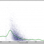
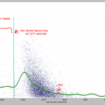
I put all the points on a scatter plot. I trained an SVR on them, so I could also show a pretty line (in green). You can see my record on the chart as a red point.

You can see some fishy stuff on the chart. The fishiest is the group of points very similar to the 10k World Record (26:17 or 1577 seconds). I looked over a couple of the tracks that generated those points and they seem to be mislabeled bike rides. Yet, I can’t explain why there are so many points around the world record value. Most likely a Strava bug.

There are a lot of people faster than the World Record. Some of them are going up to over 500 kmph. Mislabeled… flight?

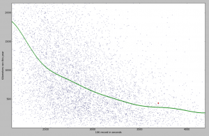
Let’s zoom on the area with the highest concentration of points. It looks like this:
strava-chart3

What you can notice from this chart:
– if you train more, you get faster. The improvement is not linear – it takes more training to improve the better you become;
– I am indeed slower than other people with similar training.

The SVR model estimated an average runner, having the same training as me, would be 5 minutes faster. Another result from the model: I would need 867km of running in order to reach a time of 50 minutes. Hmm… seems science is telling me to move on to a new sport.

All code is available on Github.

Trees, Ridges and Bulldozers made in 1000 AD

New Kaggle contest! Estimating auction price for second hand construction equipment. Didn’t know bulldozer auctions were such a big thing. We had lots of historical data (400000 auctions, starting from 1989) and we had to estimate prices a few months “into the future” (2012).

Getting to know the data

Data cleaning is a very important step when analyzing most datasets, including this one. There were a lot of noisy values. For example, a lot of the equipment appeared to have been made in the year 1000. I’m no expert in bulldozers, but the guys who are (providing us the data) told us that’s noise. So, to help the competitors, they provided an index with info regarding each bulldozer in the dataset. After “correcting” the train/test data using the index, I got worse results for my model. In the end, I used the index only for filling in missing values. Other competitors used the original data along with the index data – that might have worked a little better.

Building the model

My first model was composed out of two Random Forest Regressors and two Gradient Boosting Regressors (python using sklearn), averaged using equal weights. The parameters were set by hand, after very little testing.

A first idea of improving came after noticing a lot of the features were relative to the bulldozer category. There were six categories: ‘Motorgrader’, ‘Track Type Tractor, Dozer’, ‘Hydraulic Excavator, Track’, ‘Wheel Loader’, ‘Skid Steer Loader’ and ‘Backhoe Loader’. So I segmented the data by category and trained instances of the first model (2 RFR + 2 GBR) on each subset. This generated a fair improvement.

I continued on this line by segmenting the data even more, based on subcategory. There were around 70 subcategories. Again, segmenting and training 70 models generated another improvement. By this time, the first model (trained on the whole data), wasn’t contributing at all compared to the other two, so I removed it from the equation. With this setup, I was on 10th place on the public leaderboard one week before the end of the competition. The hosts released the leaderboard dataset, so we could also train on it, and froze the leaderboard (no use for it when you can train on the leaderboard data).

Putting the model on steroids

Usually, when you want to find the best parameters for a model, you do grid search. For my “2 RFR + 2 GBR” model, I just tested a few parameters by hand. Time to put the Core i7 to work! But instead of grid seach, which tries all combinations and keeps the best, I tried all combinations and kept the best 20-30. Afterwards, I combined them using a linear model (in this case – Ridge Regression).

I also tried other models (besides RFR and GBR) to add to the cocktail. While nothing even approached the performance GBR was getting, some managed to improve the overall score. I kept NuSVR and Lasso, also trained on (sub)categories.

Outcome and final thoughts

Based on my model’s improvement over the final week (the one with the frozen leaderboard) and my estimation over my competitors’ improvements, I expected a final ranking of 5th – 7th. Unfortunately, I came 16th. I’ve made two errors in my process:

The first one was the improper use of the auction year when training. This generated a bias in the model. Usually, I was training on auctions that took place until 2010 and trained on auctions from 2011. Nothing wrong here. Then I also trained on actions until 2011 and tested on the first part of 2012 (public leaderboard data). Nothing wrong here. For the final model, I trained on the auctions until the first part of 2012 and tested on the second part of 2012. BOOM!

Prices fluctuate a lot during the year. They are usually higher during spring and lower during fall. When I was training on data from a whole year, there was no bias for that year, since it was a value the model hasn’t seen in training. But when I tested on fall data from 2012 on a model trained using spring data from that same year, the estimated prices were a little higher.

The second error was with averaging the 20-30 small models trained on (sub)categories. In a previous contest I used neural networks for this, but the final score fluctuated too much for my taste. I also tested genetic algorithms, but I thought the scores were not very good. Ridge regression gave significantly better results. There was one small problem though: it assigned positive as well as negative weights. Usually, ensembling weights are positive and sum to one. So price estimates are averages from a lot of predictions and they generalize well to unseen cases. With negative weights, estimates are no longer averages and generalizing gets a little unpredictable.

For posterity, the code is here. I recommend checking out the winning approaches on the competition’s forum.

Event Recommendation Contest on Kaggle

The Event Recommendation Engine Challenge just finished on Kaggle.com. I managed to build a good model and finished 7th.

Given a dataset of users and events, we had to predict which event users will be interested in. We were given 38000 users, 3 million events and a bunch of data about them (like friends, attendance or interest in events).

First thing, preprocess the data and put it in a database. I had to go for a database since I couldn’t fit everything in RAM. I chose MongoDB because it’s just so easy to set up. It wasn’t the best database choice for this task. I should try and experiment with Neo4j in the future.

Regarding preprocessing, the most I’ve struggled with was location. Most users had an unformatted location string. Around half of the events had a well formatted location (city, state and country), as well as GPS coordinates. At first, I used the Yahoo Placemaker API to convert user locations into coordinates. This way, I could compute distances between users and events.

I then noticed that external data is not allowed. No problem. With 1.6 million events having both location strings and GPS coordinates, I was able to build a database of spatial information. I could then match user locations and get some coordinates without an external API.

Given a (user, event) pair, these were the features I’ve used in my model:

  • number of users attending, not attending, maybe attending and invited to the event;
  • number of friends attending, not attending, maybe attending and invited to the event;
  • location similarity between user and event;
  • number of users attending the event that have also attended events the user did;
  • similarity between the event and events the user attended, based on clusters – I used KMeans (loving scikit-learn) to cluster together similar events, based on words; I chose a few values for the number of clusters, in order to capture a little granularity;
  • same thing for events attended by friends;
  • same thing for events the user (or his friends) didn’t attend to;
  • time to event, apparently most important feature;
  • similarity between the event’s word distribution and the average distribution of words for events the user attended;
  • if the user was invited or not.

I didn’t manage to get anything out of user age and gender. I’m still wondering if (and how) that info can be used in some useful way.

In order to generate results, I went for the classifier approach (two classes, interested and not interested). I also tried ranking and regression, but classifying worked best. I chose a Random Forest (again.. scikit-learn), because it was able to work with missing values. I also added Logistic Regression (on the features that didn’t have missing values) and averaged the results.

The full code is on github. Mind you, except the scripts main.py and model.py, all other files contain code snippets I built on the fly while exploring the data in ipython.