ML Workshop at Codiax: BERT, Gradient Boosting and Journalism

Held a workshop today at Codiax 2011 with the title: Matching Journalists with Domain Experts: Text Classification with BERT and Gradient Boosting Trees from Idea to Production.

Abstract: We’ll start with a real world challenge: matching journalists interested in writing a story with relevant domain experts. We’ll examine the business use case, convert it into a technical one and discuss a baseline approach. We’ll then work on implementing a better and smarter solution, using a combination of Machine Learning algorithms. We’ll discuss performance, pros and cons, as well as future steps.

I’ve added the slides (written in jupyter notebook using the RISE extension), along with the support files, on Github: https://github.com/andreiolariu/codiax_workshop

Top Ten Finish in the Deep Learning HackerEarth Challenge

If you’re reading this, you probably know I’m a big fan of Kaggle. Unfortunately, getting good results in their contests requires a significant time investment, and I’ve lacked free time lately. But when Catalin Tiseanu‘s proposition to join the Deep Learning HackerEarth Challenge overlapped with an easier period at work, I said sure. The contest was only one month long and it was already half way in, so it was a small time commitment. I also brought my colleague Alexandru Hodorogea in as well.

First off, a few words about HackerEarth’s platform. OMG! You realize just how finessed Kaggle is in comparison. Just to read the challenge statement, you need to have an account and set up a team. That explains why they have over 4000 competitors, yet only ~200 that actually submitted something. If two people have both read the statement and want to form a team, well.. they can’t. Team merging is allowed, just not possible given the primitive interface. One of them will have to create another account. They have no forum, so it’s hard to have a conversation, share something, discuss ideas. The organizers are very slow (publishing the final leaderboard took about 10 days, posting the winning solutions still hasn’t happened and it’s been one month since it ended).

On top of that, the challenge’s dataset is freely available online. Of course, the rules forbid using any external data. The organizers mentioned they’ll manually review the code for the winning models. Still, most people are not in this for the money, so having somebody get a perfect score was inevitable. While these are easy to prune, you can still use the dataset in many less obvious ways, making the leaderboard meaningless.

A few words about the data: the training set consists of 3200 images in 25 classes. Another 1700 are in the test set. The images are conveniently small (256×256), usually of good quality, but sometimes blurry or not very clear. I think a human annotator would struggle a bit figuring out what type of product is featured in each photo.

Even though they forbid external data, the rules allow using pretrained models, and that’s how we started. We used Keras because:
– it’s very easy to use
– it comes packed with high quality pretrained models; I still can’t believe how easy they are to use; you can have a state-of-the-art model up and running in 10 lines of code
– it’s used in Jeremy Howard’s MOOC (although he mentioned he’s going to migrate the code to Pytorch)

You’ve probably guessed this competition requires some serious processing power. On my GTX 760 GPU, getting one model to something usable (~90%) took about 50 hours. Fortunately, Catalin had access to a Tesla K80, which was about 5 times faster. Not only that, but it had 2 cores, so we could work in parallel. That really helped us, especially once we got to the ensembling part.

Before going into what we did and why we did it, here is the code. Going through it very fast, we have:
– a script for preparing the data (preprocess_data.py dooh)
– a collection of useful functions (util.py)
– several scripts for training some networks (inc_agg_aug_full.py, inc_agg_aug_full_part_2.py and hodor_resnet.py)
– the ensembling script (ensemble.py)

Finetuning a pretrained Keras model would get you to about 80% on the leaderboard. Let’s see how we got to 95%. First thing – do data augmentation. This is even more important here since the dataset is very small (3200 images, with some classes having less than 100 images). We used imgaug and cranked up the knobs as long as our networks were able to learn the data. On the most aggressive setup, an input image (top left corner) would get distorted to what you see below. Surprisingly, the networks were able to generalize to the test data (despite some overfitting).

Aggressive augmentation got us to around 90-91% for a single network. We managed to push this by an extra ~1% by doing test-time augmentation. Instead of passing each test image once, we generated 10 augmentations and averaged the scores.

Finally, ensembling brought the final ~2% on the table. We didn’t have time to generate a large variety of models, so we did “poor man’s ensembling”: we added a series of checkpoints in the final stages of training a network, so we’d have not one, but several slightly different networks after training finished.

Something we put a lot of effort in, but didn’t work, was pseudolabeling. The idea is simple: train network A on the train data and evaluate on the test data. Then use both the train and test data (with the predicted labels) to train network B. Finally, use network B to generate the final predictions on the test data. We tried several approaches here, but neither worked and we don’t have an understanding of why it works on some problems and not on others.

Overall, it was a good learning opportunity for us: finetuning pretrained CNN models, working as a team across different time zones, managing GPU resources given a tight deadline and seeing how far we can push a Jupyter Notebook server until we crash it (not very far apparently).

PS: Be sure to check out Catalin’s notes here.

Mining the Best Cycling Roads around Bucharest with Strava

This year I tried to do a little more cycling during the week. I have a road bike, so I’m interested in quality roads – good tarmac, no potholes, enough shoulder to allow trucks to overtake me and live to talk about it. But I don’t know all roads around Bucharest. Best roads for biking are the smaller ones, with little traffic, that lead nowhere important. How can I find them?

I’ve worked on Strava data before and I saw here an opportunity to do it again. Using this simple script, I downloaded (over the course of several days) a total of 6 GB of GPS tracks. I started with the major Strava bike clubs in Bucharest, took all their members, then fetched all rides between April and the middle of June. Starting from 9 clubs, I looked over 1414 users. Only 674 have biked during the analyzed period. The average number of rides for those two and a half months was 25, with the [10, 25, 50, 75, 90]-percentile values of [2, 6, 17, 36, 64]. These are reasonable values, considering there are people that are commuting by bike (even over 20 km per day).

Ok, how can you determine the road quality from 6 GB of data? Simplest solution: take the speed every second (you already have that from Strava) and put it on a map. I did this by converting (lat, lng) pairs to (x, y) coordinates on an image. Each pixel was essentially a bucket, holding a list of speed values.

Let’s check out the area around Bucharest (high res version available here):

chart_all_small

In this chart, bright green lines signal roads where there are many riders going over 35 kmph (technically speaking, the 80th percentile is at 35). On the opposite side, red roads are those where you’ll be lucky going with 25 kmph. The color intensity signals how popular a route is, with rarely used roads being barely visible. I already knew the good roads north of Bucharest, with Moara Vlasiei, Dascalu, Snagov and Izvorani. I saw on Strava that the SE ride to Galbinasi is popular, but I’ve never ridden it. From this analysis, I can see there are many good roads to the south and a couple of segments to the west. Unfortunately for me, for anything that’s not in the north I have to cross Bucharest, which is a buzzkill. Also notice the course from Prima Evadare (the jagged red line in the north) and the MTB trails in Cernica, Baneasa and Comana.

Let’s zoom in a little and see how the city looks like:

chart

For this chart, I relaxed the colors a little, with 35 kmph for green and only 20 kmph for red. Things to notice:

  • the RedBull MoonTimeBike course in Tineretului (in red); notice that the whole of Tineretului or Herastrau are red; it means you can’t (and shouldn’t) bike fast in parks; please don’t bike fast in parks, it’s unpleasant (and dangerous) for bikers and pedestrians alike
  • the abandoned road circuit in Baneasa (in bright green)
  • National Arena in green
  • the two slopes around The People’s Palace in green (from how it’s built, all slopes will be green, which is not a problem, since Bucharest is pretty much flat)

Full code available here.

7th Place in Kaggle’s Driver Telematics Challenge

Intro
The purpose of the AXA Driver Telematics Challenge was to discover outliers in a dataset of trips. We were given a total of 2730 drivers, each with 200 trips. We were told that a few of those 200 trips per driver weren’t actually his and the task was to identify which ones. Somewhat similar to authorship attribution on texts.

A drive was composed of a series of GPS measurements taken each second. Each drive started at (0, 0) and all the other points were given relative to the origin, in meters. In order to make it harder to match trips to road networks, the trips were randomly rotated and parts from the start and the end were removed.

If the dataset would have been composed of only one driver, then this would actually be outlier detection. But more drivers means more information available. Using a classification approach makes it possible to incorporate that extra info.

System Overview
Local Testing
For each driver, take 180 trips and label them as 1s. Take 180 trips from other drivers and label them as 0s. Train and test on the remaining 20 trips from this driver and on another 20 trips from other drivers. That’s it.

Can we improve on this? Yes. Take more than just 180 trips from other drivers. Best results I’ve got were with values between 4×180 and 10×180. In order to avoid an unbalanced training set, I also duplicated the data from the current driver.

Considering there were trips from other drivers that I was labeling as 1s when testing locally, it wasn’t possible to get the same score locally as on the leaderboard. Yet the difference between the two scores was very predictable, at around 0.045, with variations of around 0.001. The only times I was unsure of my submissions were when I had a data sampling bug and when I tried a clustering approach using the results from local testing.

Leaderboard Submissions
Pretty much the same logic as above. Train on 190 trips from this driver, along with 190 trips from other drivers, test on the remaining 10 trips from this driver. Repeat 20 times, in order to cover all trips (similar to crossvalidation). If the process was too slow, then repeat 10 times with 180+20 splits. Also apply the data enlargement trick used in local testing.

Ensembling
In production systems, you usually try to balance the system’s performance with the computational resources it needs. In Kaggle competitions, you don’t. Ensembling is essential in getting top results. I used a linear model to combine together several predictions. The Lasso model in sklearn gave the best results, mainly because it is able to compute nonnegative weights. Having a linear blend with negative weights is just wrong.

Caching
When you have an ensemble (but not only then), you will need the same results again and again for different experiments. Having a system for caching results will make your life easier. I cached results for each model, both for local validation, as well as leaderboard submissions. With some models needing a couple of days to run (with 4 cores at 100%), caching proved useful.

Feature Extraction
Trip Features
These were the best approaches overall, with a maximum local score of 0.877 using Gradient Boosting Trees (that would be an estimated LB score of about 0.922). Some of the features used were histograms and percentiles over speeds, accelerations, angles, speed * angles, accelerations over accelerations, speeds and accelerations over larger windows.

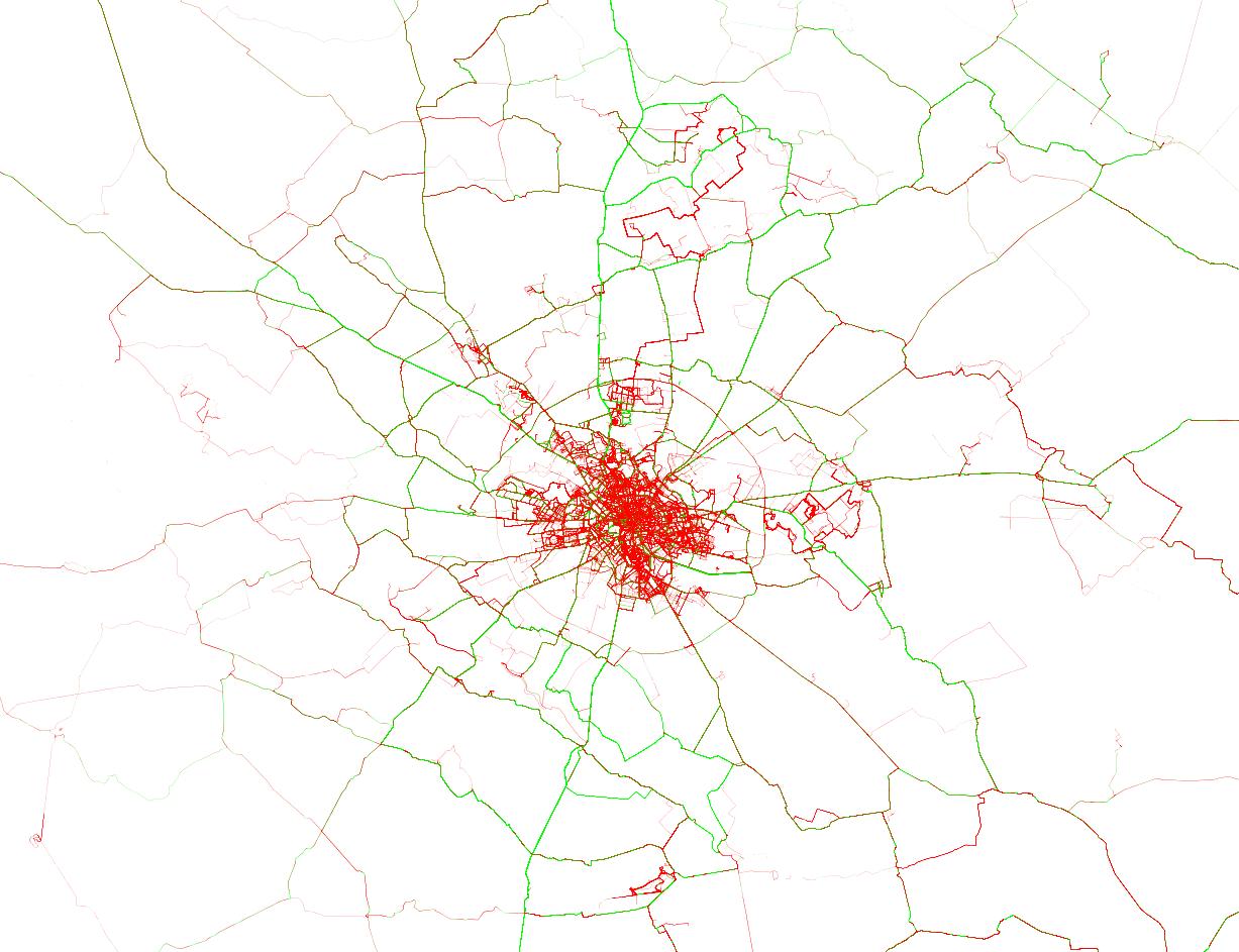
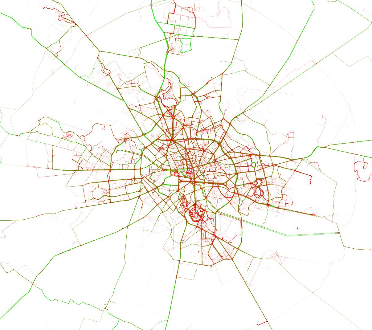
Road segment features
I’ve seen a lot of talk on the forum of matching trips using Euclidean distance. I tried to go a little further and detect similar road segments. This approach should detect repeated trips, but it should also detect if different trips have certain segments in common. I applied a trajectory simplification algorithm (Ramer-Douglas-Peucker available for Python here), then I binned the resulting segments and applied SVMs or Logistic Regression, like on a text corpus. Local results went up to 0.812 (estimated LB score of around 0.857).

One thing I didn’t like about the RDP algorithm was how similar curves could be segmented differently due to how the threshold used by the algorithm was affected by GPS noise. So I built another model. I thought the best way to encode a trip was as a list of instructions, similar to Google Maps directions. I looked at changes in heading, encoding them as left or right turns. This model scored up to 0.803 locally, lower than the RDP model, but in the final ensemble it got a bigger weight.

Movement features
I think these types of features best capture somebody’s driving style, although to some degree they also capture particular junction shapes and other road features. The main idea is to compute a few measurements each second, bin them, then treat them as text data and apply SVMs or Logistic Regression. For example, the best scoring model in this category (local score of just under 0.87) binned together the distances and the angles computed over 3-second intervals on smoothed versions of the trips (smoothing done using the Savitzky-Golay filter in scipy). After binning and converting to text data, I applied Logistic Regression on n-grams, with n between 1 and 5.

I tested over 100 individual models to select a final ensemble of 23 models. Local score was 0.9195 and the final LB score was 0.9645 (public LB), 0.9653 (private LB).

My code is available on GitHub.