Top Ten Finish in the Deep Learning HackerEarth Challenge

If you’re reading this, you probably know I’m a big fan of Kaggle. Unfortunately, getting good results in their contests requires a significant time investment, and I’ve lacked free time lately. But when Catalin Tiseanu‘s proposition to join the Deep Learning HackerEarth Challenge overlapped with an easier period at work, I said sure. The contest was only one month long and it was already half way in, so it was a small time commitment. I also brought my colleague Alexandru Hodorogea in as well.

First off, a few words about HackerEarth’s platform. OMG! You realize just how finessed Kaggle is in comparison. Just to read the challenge statement, you need to have an account and set up a team. That explains why they have over 4000 competitors, yet only ~200 that actually submitted something. If two people have both read the statement and want to form a team, well.. they can’t. Team merging is allowed, just not possible given the primitive interface. One of them will have to create another account. They have no forum, so it’s hard to have a conversation, share something, discuss ideas. The organizers are very slow (publishing the final leaderboard took about 10 days, posting the winning solutions still hasn’t happened and it’s been one month since it ended).

On top of that, the challenge’s dataset is freely available online. Of course, the rules forbid using any external data. The organizers mentioned they’ll manually review the code for the winning models. Still, most people are not in this for the money, so having somebody get a perfect score was inevitable. While these are easy to prune, you can still use the dataset in many less obvious ways, making the leaderboard meaningless.

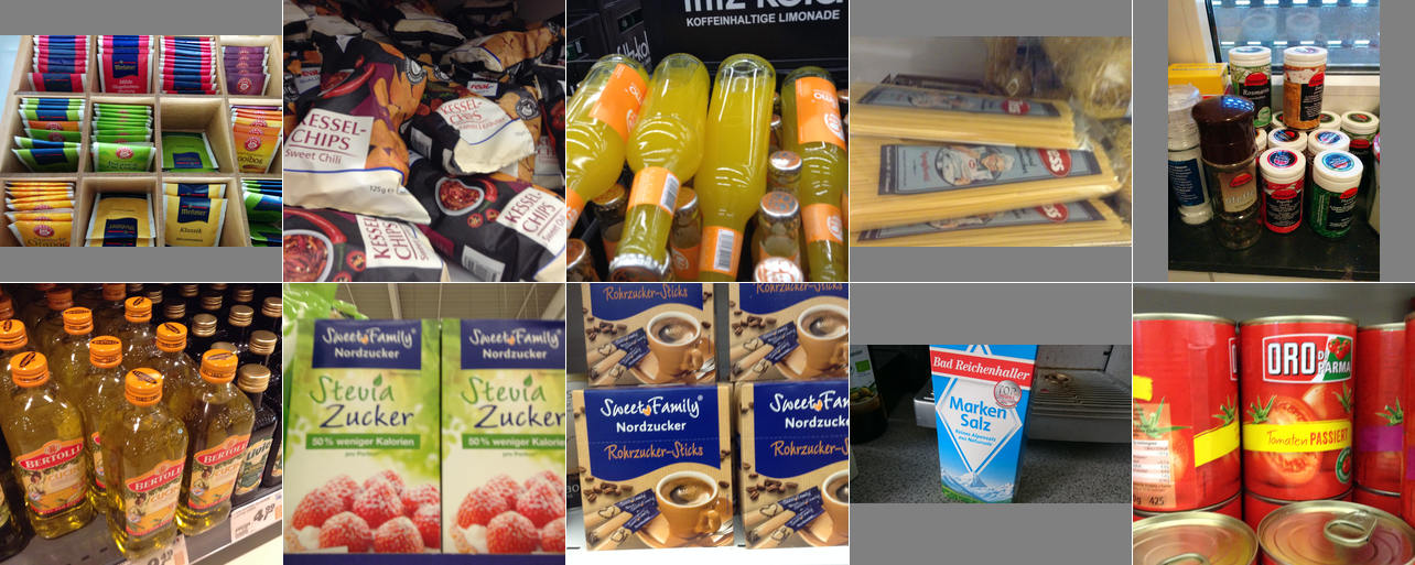
A few words about the data: the training set consists of 3200 images in 25 classes. Another 1700 are in the test set. The images are conveniently small (256×256), usually of good quality, but sometimes blurry or not very clear. I think a human annotator would struggle a bit figuring out what type of product is featured in each photo.

Even though they forbid external data, the rules allow using pretrained models, and that’s how we started. We used Keras because:
– it’s very easy to use
– it comes packed with high quality pretrained models; I still can’t believe how easy they are to use; you can have a state-of-the-art model up and running in 10 lines of code
– it’s used in Jeremy Howard’s MOOC (although he mentioned he’s going to migrate the code to Pytorch)

You’ve probably guessed this competition requires some serious processing power. On my GTX 760 GPU, getting one model to something usable (~90%) took about 50 hours. Fortunately, Catalin had access to a Tesla K80, which was about 5 times faster. Not only that, but it had 2 cores, so we could work in parallel. That really helped us, especially once we got to the ensembling part.

Before going into what we did and why we did it, here is the code. Going through it very fast, we have:
– a script for preparing the data (preprocess_data.py dooh)
– a collection of useful functions (util.py)
– several scripts for training some networks (inc_agg_aug_full.py, inc_agg_aug_full_part_2.py and hodor_resnet.py)
– the ensembling script (ensemble.py)

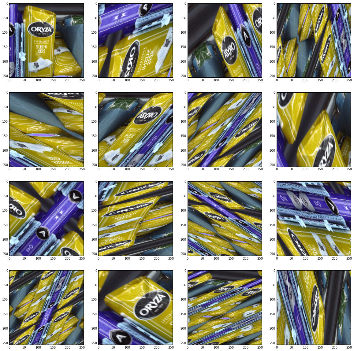
Finetuning a pretrained Keras model would get you to about 80% on the leaderboard. Let’s see how we got to 95%. First thing – do data augmentation. This is even more important here since the dataset is very small (3200 images, with some classes having less than 100 images). We used imgaug and cranked up the knobs as long as our networks were able to learn the data. On the most aggressive setup, an input image (top left corner) would get distorted to what you see below. Surprisingly, the networks were able to generalize to the test data (despite some overfitting).

Aggressive augmentation got us to around 90-91% for a single network. We managed to push this by an extra ~1% by doing test-time augmentation. Instead of passing each test image once, we generated 10 augmentations and averaged the scores.

Finally, ensembling brought the final ~2% on the table. We didn’t have time to generate a large variety of models, so we did “poor man’s ensembling”: we added a series of checkpoints in the final stages of training a network, so we’d have not one, but several slightly different networks after training finished.

Something we put a lot of effort in, but didn’t work, was pseudolabeling. The idea is simple: train network A on the train data and evaluate on the test data. Then use both the train and test data (with the predicted labels) to train network B. Finally, use network B to generate the final predictions on the test data. We tried several approaches here, but neither worked and we don’t have an understanding of why it works on some problems and not on others.

Overall, it was a good learning opportunity for us: finetuning pretrained CNN models, working as a team across different time zones, managing GPU resources given a tight deadline and seeing how far we can push a Jupyter Notebook server until we crash it (not very far apparently).

PS: Be sure to check out Catalin’s notes here.

7th Place in Kaggle’s Driver Telematics Challenge

Intro
The purpose of the AXA Driver Telematics Challenge was to discover outliers in a dataset of trips. We were given a total of 2730 drivers, each with 200 trips. We were told that a few of those 200 trips per driver weren’t actually his and the task was to identify which ones. Somewhat similar to authorship attribution on texts.

A drive was composed of a series of GPS measurements taken each second. Each drive started at (0, 0) and all the other points were given relative to the origin, in meters. In order to make it harder to match trips to road networks, the trips were randomly rotated and parts from the start and the end were removed.

If the dataset would have been composed of only one driver, then this would actually be outlier detection. But more drivers means more information available. Using a classification approach makes it possible to incorporate that extra info.

System Overview
Local Testing
For each driver, take 180 trips and label them as 1s. Take 180 trips from other drivers and label them as 0s. Train and test on the remaining 20 trips from this driver and on another 20 trips from other drivers. That’s it.

Can we improve on this? Yes. Take more than just 180 trips from other drivers. Best results I’ve got were with values between 4×180 and 10×180. In order to avoid an unbalanced training set, I also duplicated the data from the current driver.

Considering there were trips from other drivers that I was labeling as 1s when testing locally, it wasn’t possible to get the same score locally as on the leaderboard. Yet the difference between the two scores was very predictable, at around 0.045, with variations of around 0.001. The only times I was unsure of my submissions were when I had a data sampling bug and when I tried a clustering approach using the results from local testing.

Leaderboard Submissions
Pretty much the same logic as above. Train on 190 trips from this driver, along with 190 trips from other drivers, test on the remaining 10 trips from this driver. Repeat 20 times, in order to cover all trips (similar to crossvalidation). If the process was too slow, then repeat 10 times with 180+20 splits. Also apply the data enlargement trick used in local testing.

Ensembling
In production systems, you usually try to balance the system’s performance with the computational resources it needs. In Kaggle competitions, you don’t. Ensembling is essential in getting top results. I used a linear model to combine together several predictions. The Lasso model in sklearn gave the best results, mainly because it is able to compute nonnegative weights. Having a linear blend with negative weights is just wrong.

Caching
When you have an ensemble (but not only then), you will need the same results again and again for different experiments. Having a system for caching results will make your life easier. I cached results for each model, both for local validation, as well as leaderboard submissions. With some models needing a couple of days to run (with 4 cores at 100%), caching proved useful.

Feature Extraction
Trip Features
These were the best approaches overall, with a maximum local score of 0.877 using Gradient Boosting Trees (that would be an estimated LB score of about 0.922). Some of the features used were histograms and percentiles over speeds, accelerations, angles, speed * angles, accelerations over accelerations, speeds and accelerations over larger windows.

Road segment features
I’ve seen a lot of talk on the forum of matching trips using Euclidean distance. I tried to go a little further and detect similar road segments. This approach should detect repeated trips, but it should also detect if different trips have certain segments in common. I applied a trajectory simplification algorithm (Ramer-Douglas-Peucker available for Python here), then I binned the resulting segments and applied SVMs or Logistic Regression, like on a text corpus. Local results went up to 0.812 (estimated LB score of around 0.857).

One thing I didn’t like about the RDP algorithm was how similar curves could be segmented differently due to how the threshold used by the algorithm was affected by GPS noise. So I built another model. I thought the best way to encode a trip was as a list of instructions, similar to Google Maps directions. I looked at changes in heading, encoding them as left or right turns. This model scored up to 0.803 locally, lower than the RDP model, but in the final ensemble it got a bigger weight.

Movement features
I think these types of features best capture somebody’s driving style, although to some degree they also capture particular junction shapes and other road features. The main idea is to compute a few measurements each second, bin them, then treat them as text data and apply SVMs or Logistic Regression. For example, the best scoring model in this category (local score of just under 0.87) binned together the distances and the angles computed over 3-second intervals on smoothed versions of the trips (smoothing done using the Savitzky-Golay filter in scipy). After binning and converting to text data, I applied Logistic Regression on n-grams, with n between 1 and 5.

I tested over 100 individual models to select a final ensemble of 23 models. Local score was 0.9195 and the final LB score was 0.9645 (public LB), 0.9653 (private LB).

My code is available on GitHub.

Trees, Ridges and Bulldozers made in 1000 AD

New Kaggle contest! Estimating auction price for second hand construction equipment. Didn’t know bulldozer auctions were such a big thing. We had lots of historical data (400000 auctions, starting from 1989) and we had to estimate prices a few months “into the future” (2012).

Getting to know the data

Data cleaning is a very important step when analyzing most datasets, including this one. There were a lot of noisy values. For example, a lot of the equipment appeared to have been made in the year 1000. I’m no expert in bulldozers, but the guys who are (providing us the data) told us that’s noise. So, to help the competitors, they provided an index with info regarding each bulldozer in the dataset. After “correcting” the train/test data using the index, I got worse results for my model. In the end, I used the index only for filling in missing values. Other competitors used the original data along with the index data – that might have worked a little better.

Building the model

My first model was composed out of two Random Forest Regressors and two Gradient Boosting Regressors (python using sklearn), averaged using equal weights. The parameters were set by hand, after very little testing.

A first idea of improving came after noticing a lot of the features were relative to the bulldozer category. There were six categories: ‘Motorgrader’, ‘Track Type Tractor, Dozer’, ‘Hydraulic Excavator, Track’, ‘Wheel Loader’, ‘Skid Steer Loader’ and ‘Backhoe Loader’. So I segmented the data by category and trained instances of the first model (2 RFR + 2 GBR) on each subset. This generated a fair improvement.

I continued on this line by segmenting the data even more, based on subcategory. There were around 70 subcategories. Again, segmenting and training 70 models generated another improvement. By this time, the first model (trained on the whole data), wasn’t contributing at all compared to the other two, so I removed it from the equation. With this setup, I was on 10th place on the public leaderboard one week before the end of the competition. The hosts released the leaderboard dataset, so we could also train on it, and froze the leaderboard (no use for it when you can train on the leaderboard data).

Putting the model on steroids

Usually, when you want to find the best parameters for a model, you do grid search. For my “2 RFR + 2 GBR” model, I just tested a few parameters by hand. Time to put the Core i7 to work! But instead of grid seach, which tries all combinations and keeps the best, I tried all combinations and kept the best 20-30. Afterwards, I combined them using a linear model (in this case – Ridge Regression).

I also tried other models (besides RFR and GBR) to add to the cocktail. While nothing even approached the performance GBR was getting, some managed to improve the overall score. I kept NuSVR and Lasso, also trained on (sub)categories.

Outcome and final thoughts

Based on my model’s improvement over the final week (the one with the frozen leaderboard) and my estimation over my competitors’ improvements, I expected a final ranking of 5th – 7th. Unfortunately, I came 16th. I’ve made two errors in my process:

The first one was the improper use of the auction year when training. This generated a bias in the model. Usually, I was training on auctions that took place until 2010 and trained on auctions from 2011. Nothing wrong here. Then I also trained on actions until 2011 and tested on the first part of 2012 (public leaderboard data). Nothing wrong here. For the final model, I trained on the auctions until the first part of 2012 and tested on the second part of 2012. BOOM!

Prices fluctuate a lot during the year. They are usually higher during spring and lower during fall. When I was training on data from a whole year, there was no bias for that year, since it was a value the model hasn’t seen in training. But when I tested on fall data from 2012 on a model trained using spring data from that same year, the estimated prices were a little higher.

The second error was with averaging the 20-30 small models trained on (sub)categories. In a previous contest I used neural networks for this, but the final score fluctuated too much for my taste. I also tested genetic algorithms, but I thought the scores were not very good. Ridge regression gave significantly better results. There was one small problem though: it assigned positive as well as negative weights. Usually, ensembling weights are positive and sum to one. So price estimates are averages from a lot of predictions and they generalize well to unseen cases. With negative weights, estimates are no longer averages and generalizing gets a little unpredictable.

For posterity, the code is here. I recommend checking out the winning approaches on the competition’s forum.

Event Recommendation Contest on Kaggle

The Event Recommendation Engine Challenge just finished on Kaggle.com. I managed to build a good model and finished 7th.

Given a dataset of users and events, we had to predict which event users will be interested in. We were given 38000 users, 3 million events and a bunch of data about them (like friends, attendance or interest in events).

First thing, preprocess the data and put it in a database. I had to go for a database since I couldn’t fit everything in RAM. I chose MongoDB because it’s just so easy to set up. It wasn’t the best database choice for this task. I should try and experiment with Neo4j in the future.

Regarding preprocessing, the most I’ve struggled with was location. Most users had an unformatted location string. Around half of the events had a well formatted location (city, state and country), as well as GPS coordinates. At first, I used the Yahoo Placemaker API to convert user locations into coordinates. This way, I could compute distances between users and events.

I then noticed that external data is not allowed. No problem. With 1.6 million events having both location strings and GPS coordinates, I was able to build a database of spatial information. I could then match user locations and get some coordinates without an external API.

Given a (user, event) pair, these were the features I’ve used in my model:

  • number of users attending, not attending, maybe attending and invited to the event;
  • number of friends attending, not attending, maybe attending and invited to the event;
  • location similarity between user and event;
  • number of users attending the event that have also attended events the user did;
  • similarity between the event and events the user attended, based on clusters – I used KMeans (loving scikit-learn) to cluster together similar events, based on words; I chose a few values for the number of clusters, in order to capture a little granularity;
  • same thing for events attended by friends;
  • same thing for events the user (or his friends) didn’t attend to;
  • time to event, apparently most important feature;
  • similarity between the event’s word distribution and the average distribution of words for events the user attended;
  • if the user was invited or not.

I didn’t manage to get anything out of user age and gender. I’m still wondering if (and how) that info can be used in some useful way.

In order to generate results, I went for the classifier approach (two classes, interested and not interested). I also tried ranking and regression, but classifying worked best. I chose a Random Forest (again.. scikit-learn), because it was able to work with missing values. I also added Logistic Regression (on the features that didn’t have missing values) and averaged the results.

The full code is on github. Mind you, except the scripts main.py and model.py, all other files contain code snippets I built on the fly while exploring the data in ipython.

My first Kaggle competition (and how I ranked 3rd)

1. Intro
First, a few words about Kaggle. It’s a website/community for machine learning competitions. Companies and organizations share a problem (most of the time it’s an actual real world problem), provide a dataset and offer prizes for the best performing models. Some examples of current competitions: predict customer retention, discover dark matter by how it bends light in space photos (AWESOME), predict diseases in patients based on their history (and win $3 million!) and so on.

I was planning to join a competition on Kaggle since I found out about the website (in spring, I think), but I never found the time to. And then I got an email about a new competition – to detect insults in comments. I had a little knowledge on text mining, I also had some free time, so I downloaded the dataset and started coding.

Impermium, the company behind this competition, came with some prize money. First place got $7000, while second place got $2500. Third place got just the eternal glory, yay!

For implementation, I used python, the wonderful scikit-learn library (for the SVM implementation) and the neurolab library (for the neural network implementation).

2. General System Architecture
Here I’ll briefly describe the architecture of the model that performed the best. This architecture will be expanded afterwards.

First, all texts were preprocessed. Then they were fed into 3 different classifiers: word-level SVM, character-level SVM and a dictionary-based classifier. The output from each classifier, along with some other features, were fed into a neural network.

3. Tokenizing
This step was a lot more important than I first imagined. Here are some of the things that I tried and improved (or at least seemed to) the model score:
– removing links, html entities and html code
– formatting whitespaces (removing duplicates, removing newlines and tabs)
– removing non-ascii characters (I didn’t think people curse using special characters; I would reconsider this decision, given more time)
– adding special tokens in texts for character groups such as: #$%#$ (some people curse like this), ?!???, !!!!!!
– removing repeated letters: coooool -> cool, niiiice -> niice (yes, this is not the best implementation, but it usually works)
– replacing smileys by 2 tokens, one for positive smileys and one for negative smileys (“saddies”?)
– removing dots inside words (some people put dots inside curse words – they’re not getting away with this!)
– grouping together sequences of one-letter words – like “f u c k” (some people split a curse word in letters – they’re not getting away with it!)
– trying to group consecutive words (like “fu ck”) using a dictionary (some people split curse words in 2 – they’re not getting away with it!)

4. Classifiers
The first classifier was an SVM on word ngrams, with n from 1 to 4. Not a lot can be said here, I just imported it, fed it the ngrams generated from the tokenized text and let scikit-learn do its stuff.

The second classifier was another SVM, this time on character ngrams, with n from 4 to 10.

The third classifier was a custom build dictionary based classifier. It used a curse words dictionary (which I found online and then enriched with words I found in the misclassified examples). This classifier just looked if the text had words from the dictionary and also words like “you”, “your”, “yourself” (which you use when cursing somebody). It then computed a simple score based on the distances between the curse words and the “you”-words.

The final classifier was used to combine the previous ones. I used a neural network, but I’m sure other techniques can be applied here. The network had a hidden layer of 3 neurons and was trained using the function “train_rprop” (from the neurolab library). I took advantage of the network’s flexibility and added some more features as inputs:
– the ratio of curse words
– the text length
– the ratio of *, ! or ?
– the ratio of capital letter (should have used words in all caps instead)

5. Epilogue
I used k-folds cross-validation for model selection (scikit-learn comes with some nifty tools here also).

In total, I worked around one week for this. I tried a lot more models and approaches, but what I’ve showed here got the best score. I’d love to share the code, but it’s written so crappily (due to some hard core time constraints) that I’m too ashamed to release it. Still, if anybody wants it, please contact me – I’ll share it after explicitly agreeing to one condition: Don’t make fun of it. Screw that, code available here.

I think 3rd place is a very good result (considering it’s my first competition ever). Still, I noticed that there were a lot of mislabeled examples (perhaps more than the 1% stated on the contest page). This might have had an influence on the final ranking (the difference between the winner’s score and the fifth score was less than 1%).

Yet again, I always say “Fortune favors the brave” (I don’t believe in luck). Jumping to some actionable information, light bending dark matter detection sounds pretty cool!